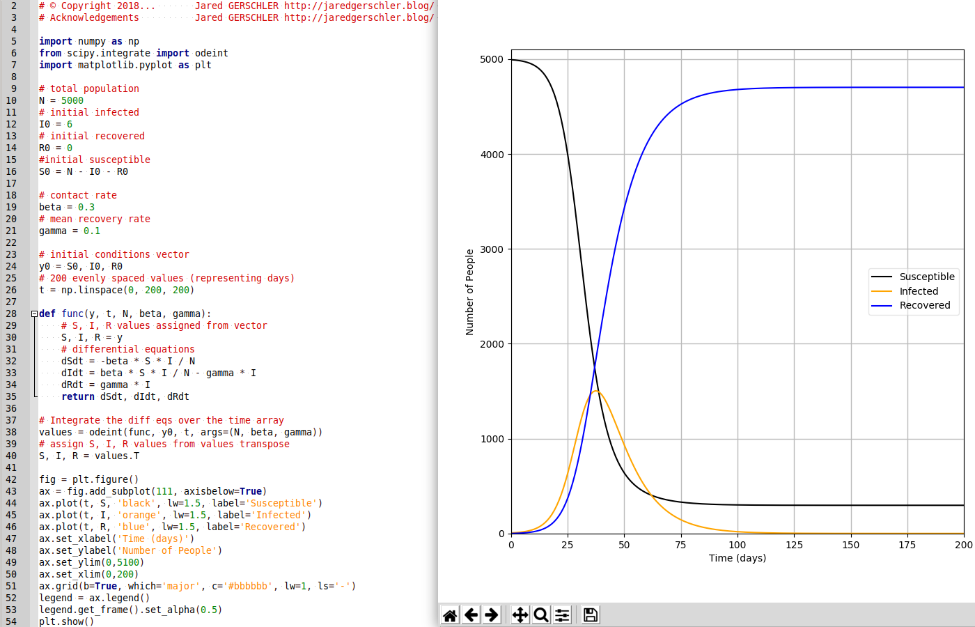
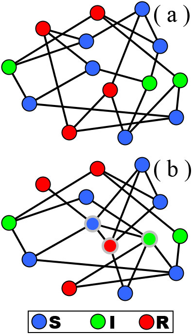
Modèle SIR programmé en Python
# coding: utf-8             Autorise les accents
# © Copyright 2018...       Jared GERSCHLER http://jaredgerschler.blog/
# Acknowledgements          Jared GERSCHLER http://jaredgerschler.blog/

import numpy as np
from scipy.integrate import odeint
import matplotlib.pyplot as plt

# total population
N = 5000
# initial infected
I0 = 6
# initial recovered
R0 = 0
#initial susceptible
S0 = N - I0 - R0

# contact rate
beta = 0.3
# mean recovery rate
gamma = 0.1

# initial conditions vector
y0 = S0, I0, R0
# 200 evenly spaced values (representing days)
t = np.linspace(0, 200, 200)

def func(y, t, N, beta, gamma):
    # S, I, R values assigned from vector
    S, I, R = y
    # differential equations
    dSdt = -beta * S * I / N
    dIdt = beta * S * I / N - gamma * I
    dRdt = gamma * I
    return dSdt, dIdt, dRdt

# Integrate the diff eqs over the time array
values = odeint(func, y0, t, args=(N, beta, gamma))
# assign S, I, R values from values transpose
S, I, R = values.T

fig = plt.figure()
ax = fig.add_subplot(111, axisbelow=True)
ax.plot(t, S, 'black', lw=1.5, label='Susceptible')
ax.plot(t, I, 'orange', lw=1.5, label='Infected')
ax.plot(t, R, 'blue', lw=1.5, label='Recovered')
ax.set_xlabel('Time (days)')
ax.set_ylabel('Number of People')
ax.set_ylim(0,5100)
ax.set_xlim(0,200)
ax.grid(b=True, which='major', c='#bbbbbb', lw=1, ls='-')
legend = ax.legend()
legend.get_frame().set_alpha(0.5)
plt.show()