Démonstrations
Hello, Website!
\(A = \pi*r^{2}\)
\[E = mc^{2}\]
Statistiques simples avec R
summary((0:9)^2)## Min. 1st Qu. Median Mean 3rd Qu. Max.
## 0.00 5.25 20.50 28.50 45.75 81.00Graphes simples avec R
# Define cars vector with 5 values
cars <- c(1, 3, 6, 4, 9)

# Define some colors ideal for black & white print
colors <- c("white","grey70","grey90","grey50","black")

# Calculate the percentage for each day, rounded to one
# decimal place
car_labels <- round(cars/sum(cars) * 100, 1)

# Concatenate a '%' char after each value
car_labels <- paste(car_labels, "%", sep="")

# Create a pie chart with defined heading and custom colors
# and labels
pie(cars, main="Cars", col=colors, labels=car_labels,
   cex=0.8)

# Create a legend at the right
legend(1.5, 0.5, c("Mon","Tue","Wed","Thu","Fri"), cex=0.8,
   fill=colors)
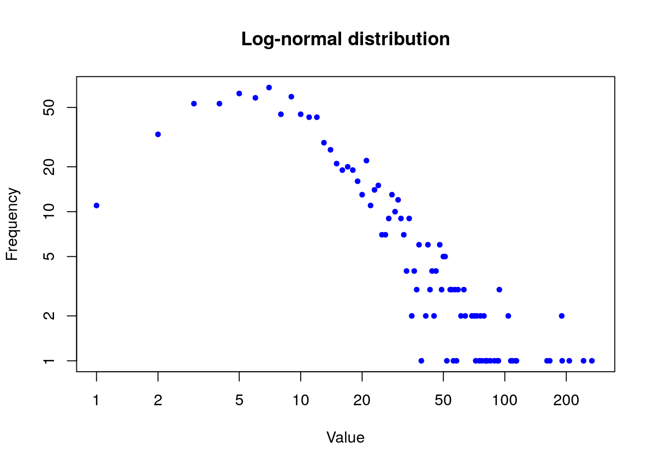
# Get a random log-normal distribution
r <- rlnorm(1000)

# Get the distribution without plotting it using tighter breaks
h <- hist(r, plot=F, breaks=c(seq(0,max(r)+1, .1)))

# Plot the distribution using log scale on both axes, and use
# blue points
plot(h$counts, log="xy", pch=20, col="blue",
    main="Log-normal distribution",
    xlab="Value", ylab="Frequency")
## Warning in xy.coords(x, y, xlabel, ylabel, log): 189 y values <= 0 omitted from
## logarithmic plot
Tableau des lettres grecques
For those of you who don’t know your Greek alphabet, it’s time to learn it : name symbol \(\LaTeX\)
| Prononciation et lettre | Prononciation et lettre | Prononciation et lettre | Prononciation et lettre |
|---|---|---|---|
| alpha \(\alpha \ A\) A | beta \(\beta \ B\) B | gamma \(\gamma \ \Gamma\) | delta \(\delta \ \Delta\) |
| epsilon \(\epsilon \ E\) E | (epsilon) \(\varepsilon \ E\) | zeta \(\zeta \ Z\) Z | eta \(\eta \ H\) |
| theta \(\theta \ \Theta\) | iota \(\iota \ I\) I | kappa \(\kappa \ K\) K | lambda \(\lambda \ \Lambda\) |
| mu \(\mu \ M\) M | nu \(\nu \ N\) N | xi \(\xi \ \Xi\) | omicron \(\omicron \ O\) O |
| pi \(\pi \ \Pi\) | rho \(\rho \ P\) P | sigma \(\sigma \ \Sigma\) | tau \(\tau \ T\) |
| upsilon \(\upsilon \ Y\) Y | phi \(\phi \ \Phi\) | (phi) \(\varphi\) | chi \(\chi \ X\) X |
| psi \(\psi \ \Psi\) | omega \(\omega \ \Omega\) | - | - |
Quelques examples d’utilisation de \(\LaTeX\) dans des documents R Markdown
R Markdown allows you to mix text, R code, R output, R graphics, and mathematics in a single document. The mathematics is done using a version of \(\LaTeX\), the premiere mathematics typesetting program. (Our textbook was done entirely in \(\LaTeX\). Getting in and out of \(\LaTeX\) mode
You enter \(\LaTeX\) mode using $latex (for inline mathematics) or \[latex (for displayed equations). You get back out of \( \LaTeX \) mode using either $ or \]. Some basic mathematics you might use
Commands in \(\LaTeX\) are preceded by a backslash (). The simplest commands simply produce a symbol: Command Result A B \(\quad\) \(A \cup B\) A B \(A \cap B\) x A \(x \in A\) 5 2 \(5 \pm 2\) (x) \(\log(x)\) (x) \(\sin(x)\)
Other commands take additional inputs (placed inside curly braces {}): Command Result \(\sqrt{27}\) \(\overline{x}\) \(\frac{x}{n}\) \(\binom{k}{n}\) \(\quad\) \(\frac{\partial f}{\partial x}\)
The underscore () and carrot (^) have special uses in \(\LaTeX\). (Note the use of to get inline mathematics set with larger fonts and more vertical space.) Command Result x^2 \(x^2\) x_2 \(x_2\) {x} \(\lim_{x \to \infty}\) _{x} \(\displaystyle \lim_{x \to \infty}\) _0^{} f(x) ; dx \(\int_0^{\infty} f(x) \; dx\) _0^{} f(x) ; dx \(\quad\) \(\displaystyle \int_0^{\infty} f(x) \; dx\) The Greek Alphabet
For those of you who don’t know your Greek alphabet, it’s time to learn it. name symbol \(\LaTeX\) alpha \(\alpha \ A\) A beta \(\beta \ B\) B gamma \(\gamma \ \Gamma\) delta \(\delta \ \Delta\) epsilon \(\epsilon \ E\) E (epsilon) \(\varepsilon \ E\) zeta \(\zeta \ Z\) Z eta \(\eta \ H\) theta \(\theta \ \Theta\) iota \(\iota \ I\) I kappa \(\kappa \ K\) K lambda \(\lambda \ \Lambda\) mu \(\mu \ M\) M nu \(\nu \ N\) N xi \(\xi \ \Xi\) omicron \(\omicron \ O\) O pi \(\pi \ \Pi\) rho \(\rho \ P\) P sigma \(\sigma \ \Sigma\) tau \(\tau \ T\) upsilon \(\upsilon \ Y\) Y phi \(\phi \ \Phi\) (phi) \(\varphi\) chi \(\chi \ X\) X psi \(\psi \ \Psi\) omega \(\omega \ \Omega\)