[∇] [@] Introduction à R et RStudio
Version 2020-10-18
Licence cc-by-sa ModLibre.info sauf autres indications
NB : Copiez les instructions que vous voulez tester dans une version récente de R ou RStudio
Hello, Website!
Dates 1
‘format(Sys.Date(), “%B %d, %Y”)’ ⇒ ‘octobre 25, 2022’
‘format(Sys.Date(), “%Y-%B-%d”)’ ⇒ ‘2022-octobre-25’
‘format(Sys.Date(), “%Y-%m-%d”)’ ⇒ ‘2022-10-25’
‘format(Sys.Date(), “%y-%m-%d”)’ ⇒ ‘22-10-25’
Statistiques simples avec R
summary((0:9)^2)## Min. 1st Qu. Median Mean 3rd Qu. Max.
## 0.00 5.25 20.50 28.50 45.75 81.00[∇] [Δ] Graphes simples avec R 2
# Define cars vector with 5 values
cars <- c(1, 3, 6, 4, 9)

# Define some colors ideal for black & white print
colors <- c("white","grey70","grey90","grey50","black")

# Calculate the percentage for each day, rounded to one
# decimal place
car_labels <- round(cars/sum(cars) * 100, 1)

# Concatenate a '%' char after each value
car_labels <- paste(car_labels, "%", sep="")

# Create a pie chart with defined heading and custom colors
# and labels
pie(cars, main="Cars", col=colors, labels=car_labels,
   cex=0.8)

# Create a legend at the right
legend(1.5, 0.5, c("Mon","Tue","Wed","Thu","Fri"), cex=0.8,
   fill=colors)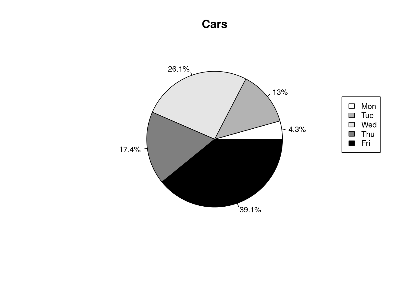
# Get a random log-normal distribution
r <- rlnorm(1000)

# Get the distribution without plotting it using tighter breaks
h <- hist(r, plot=F, breaks=c(seq(0,max(r)+1, .1)))

# Plot the distribution using log scale on both axes, and use
# blue points
plot(h$counts, log="xy", pch=20, col="blue",
    main="Log-normal distribution",
    xlab="Value", ylab="Frequency")
## Warning in xy.coords(x, y, xlabel, ylabel, log): 179 valeurs y <= 0 sont
## ignorées pour le graphe logarithmique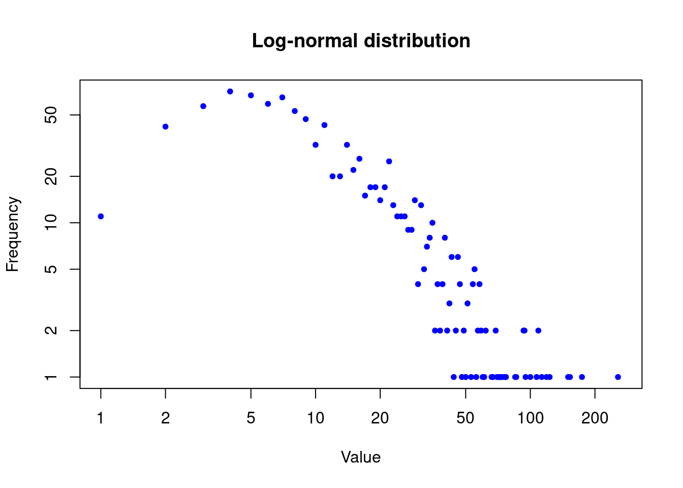
[∇] [Δ] Quelques examples d’utilisation de \(\LaTeX\) dans des documents R
R Markdown allows you to mix text, R code, R output, R graphics, and mathematics in a single document. The mathematics is done using a version of \(\LaTeX\), the premiere mathematics typesetting program. (Our textbook was done entirely in \(\LaTeX\)…) (à compléter).
\(A = \pi*r^{2}\)
\[E = mc^{2}\]
[∇] [Δ] Tableau des lettres grecques en \(\LaTeX\) 3
For those of you who don’t know your Greek alphabet, it’s time to learn it : name symbol \(\LaTeX\)
| Prononciation et lettre | Prononciation et lettre | Prononciation et lettre | Prononciation et lettre |
|---|---|---|---|
| alpha \(\alpha \ A\) A | beta \(\beta \ B\) B | gamma \(\gamma \ \Gamma\) | delta \(\delta \ \Delta\) |
| epsilon \(\epsilon \ E\) E | (epsilon) \(\varepsilon \ E\) | zeta \(\zeta \ Z\) Z | eta \(\eta \ H\) |
| theta \(\theta \ \Theta\) | iota \(\iota \ I\) I | kappa \(\kappa \ K\) K | lambda \(\lambda \ \Lambda\) |
| mu \(\mu \ M\) M | nu \(\nu \ N\) N | xi \(\xi \ \Xi\) | omicron \(\omicron \ O\) O |
| pi \(\pi \ \Pi\) | rho \(\rho \ P\) P | sigma \(\sigma \ \Sigma\) | tau \(\tau \ T\) |
| upsilon \(\upsilon \ Y\) Y | phi \(\phi \ \Phi\) | (phi) \(\varphi\) | chi \(\chi \ X\) X |
| psi \(\psi \ \Psi\) | omega \(\omega \ \Omega\) | - | - |
[∇] [Δ] Modèles d’épidémies avec R 4
Exemple : Modèle SIR Model avec une dynamique vitale (Un Groupe)
param <- param.dcm(inf.prob = 0.2, act.rate = 5,
rec.rate = 1/3, a.rate = 1/90, ds.rate = 1/100,
di.rate = 1/35, dr.rate = 1/100)
init <- init.dcm(s.num = 500, i.num = 1, r.num = 0)
control <- control.dcm(type = "SIR", nsteps = 500)
mod2 <- dcm(param, init, control)
mod2
plot(mod2)Producing Simple Graphs with R © 2006-16 by Frank McCown↩︎
Modèle SIR (Licence GPL-3)↩︎