[∇] [@] Introduction à SageMath
Version 2020-10-17
Licence cc-by-sa ModLibre.info sauf autres indications
NB : Copiez les instructions que vous voulez tester dans une version récente de SageMath
[∇] [Δ] Plan de l’introduction à SageMath
- Affichages exacts ou formatés
- Matrices
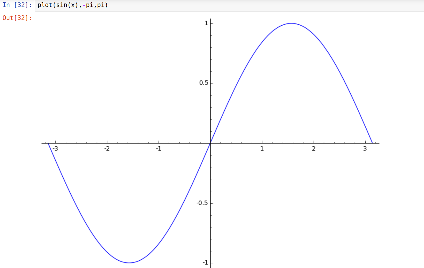
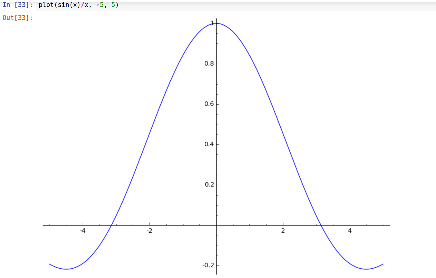
- Graphiques
- Polynomes
- Différentiation et intégration
- Théorie des graphes
- Python
- Python : Triangle de Sierpinski
- Python : Lotka-Volterra
- Langage R
- Calculs interactifs
- Calculs itératifs
- Références
- Fin
[∇] [Δ] Affichages exacts
a, b = var('a', 'b')
a^2 + b^2
a^2 + b^2
Toto = 22
Toto
22
6/43/2
8/6 4/3
[∇] [Δ] Affichages exacts : factorielles
factorial(600)12655723162254307425418678245150829297671403862274660768187828858528140823147351237817802795619571074765208532598060224803240903782164769430795025578054271906283387643826088448124626488332623608376164081221171179439885840257818732919037889603719186743943363062139593784473922231852782547619771723889252476871186000174697934549112845662596182308280390615184691924446215552586523740084932807259056238962104689731522587564412231618018774350801526839567367444928206231310973619440354723718012867753019556135721376207959558860559933052856914157120622980057169891912595926540427596853441276985006724869558201930657900240943007657817473684008944448183219124163017666607770667585082169598239230274035517738648065600492702095732843492708856036920219883363111527988109277392696562776813446645651238419301586157342867860646666350050113314787911320639668510871569846664873595017518995670958477806411667505346462590471136862647349666243426242677175204732314281064417939041868653741187423064985189556742640111598580035644021835576715752869397465453828584471291269955890393294448315746500268702149708808053100406398480942695623586049403348084970064668900206251516968479727515576425962392136269169089884609794271331061018895634421094082310408889752954265842691732460538911784960000000000000000000000000000000000000000000000000000000000000000000000000000000000000000000000000000000000000000000000000000000000000000000000000000
factorial(100)93326215443944152681699238856266700490715968264381621468592963895217599993229915608941463976156518286253697920827223758251185210916864000000000000000000000000
i = var('i')
i = int(40*random())
i, factorial(i)
(35, 10333147966386144929666651337523200000000L)
[∇] [Δ] Affichages exacts : trigonométrie
pipi
cos(pi)+10
cos(pi) + 1cos(pi) + 1
cos(pi/2)0
cos(pi/3)1/2
cos(2*pi/3)-1/2
[∇] [Δ] Affichages exacts : trigonométrie
cos(pi/17)cos(1/17*pi)
cos(pi/4)1/2*sqrt(2)
cos(pi/5)1/4*sqrt(5) + 1/4
latex(cos(pi/6)) \[\frac{1}{2} \, \sqrt{3}\]
[∇] [Δ] Affichages exacts
factorial(150)57133839564458545904789328652610540031895535786011264182548375833179829124845398393126574488675311145377107878746854204162666250198684504466355949195922066574942592095735778929325357290444962472405416790722118445437122269675520000000000000000000000000000000000000
(3/4)**327/64
sqrt(31)sqrt(31)
[∇] [Δ] Affichages numériques formatés
n(8/60)0.133333333333333
n(8/6, 53)1.33333333333333
n(8/6, 200)1.3333333333333333333333333333333333333333333333333333333333
n(8/6, digits = 6)1.33333
n(factorial(150))5.71338395644585e262
n(pi)3.14159265358979
n(pi, 53)3.14159265358979
N(pi, 200)3.1415926535897932384626433832795028841971693993751058209749
N(pi, digits = 6)3.14159
[∇] [Δ] Matrices
random_matrix(ZZ,5,5)[ -1 3 1 -1 -1] [ 1 -2 -1 -12 -2] [ 0 0 0 1 -1] [ -1 -1 0 1 1] [ 0 1 4 0 0]
random_matrix(QQ,5,5)[1/2 0 1 -2 -2] [ -1 -2 0 -1 2] [ 1 0 0 -1 0] [ 1 0 -2 2 -2] [ 1 1 0 1 0]
random_matrix(CC,5,3)[ 0.489586894030108 + 0.248333693548485I 0.925504040903679 + 0.971022768196534I -0.750224957551303 - 0.0925885687612076*I] [ 0.734730117716241 - 0.579273576679723I 0.875148233935730 + 0.709337958682879I 0.878029911308471 + 0.343286943457176*I] [ -0.424036443895202 - 0.574726880627621I -0.575904338863223 - 0.540294007216634I 0.858925895602405 - 0.711972537122582*I] [ -0.385622295725467 + 0.577951267273975I -0.742864134414032 - 0.888773779912506I 0.0601516717804098 + 0.374152600975045*I] [-0.636058406210340 + 0.0165073241401774I -0.901975628663192 - 0.755812968489364I -0.669377326258509 - 0.572944447380326*I]
random_matrix(RR,5,5)[ -0.811704668565255 0.785793156577759 0.222675354600597 -0.497374627818053 0.616438972358207] [ -0.723667981709970 -0.0614798957323899 0.671725707237411 0.431412939690882 -0.373773178121372] [ 0.332089160509406 0.346216041138981 0.312238117299918 0.0663332833178378 0.140395014475014] [ -0.463024535143201 -0.729251092252178 -0.952018423860972 -0.194440129439551 -0.572535231630911] [-0.0832055220404708 -0.120197272272354 -0.853728529304118 0.450491186112010 -0.894917056072650]
[∇] [Δ] Graphique 3D : x^2 + y^2
x, y = var('x', 'y')
plot3d(x^2 + y^2, (x,-1,1), (y,-1,1), viewer='threejs')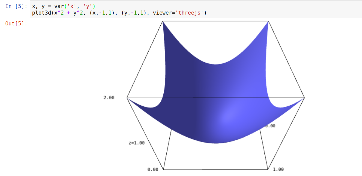
[∇] [Δ] Graphique 3D : x^2 + y^3
x, y = var('x', 'y')
plot3d(x^2 + y^3, (x,-1,1), (y,-1,1), viewer='threejs')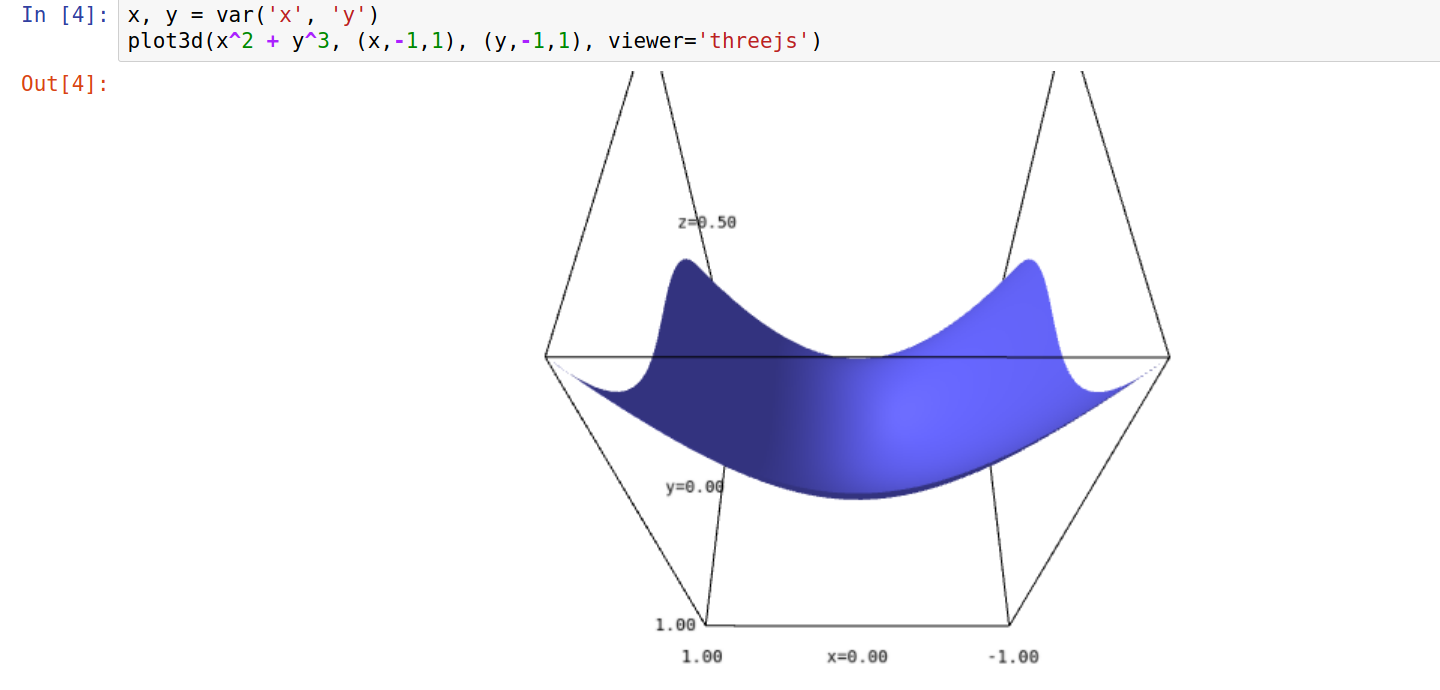
[∇] [Δ] Polynomes
    a, b = var('a, b')
P = expand( (a*x + b)^2 )
Pa^2x^2 + 2abx + b^2
factor(P)(a*x + b)^2
P.factor()(a*x + b)^2
[∇] [Δ] Différentiation et intégration
f(x) = x^2
derivative( f(x) )
2*x
# g(x) = integral( f(x))  = Ancienne forme
g(x) = integral( f(x), x)
g(x)
1/3*x^3
f(x).integral(x)1/3*x^3
integral(f(x), x, 0, 1)1/3
integral_numerical(f(x), 0, 1)(0.3333333333333333, 3.700743415417188e-15)
d(x) = derivative( f(x) )
g(x) = integral( f(x), x )
plot( (d(x), f(x), g(x)), x, 0, 1) 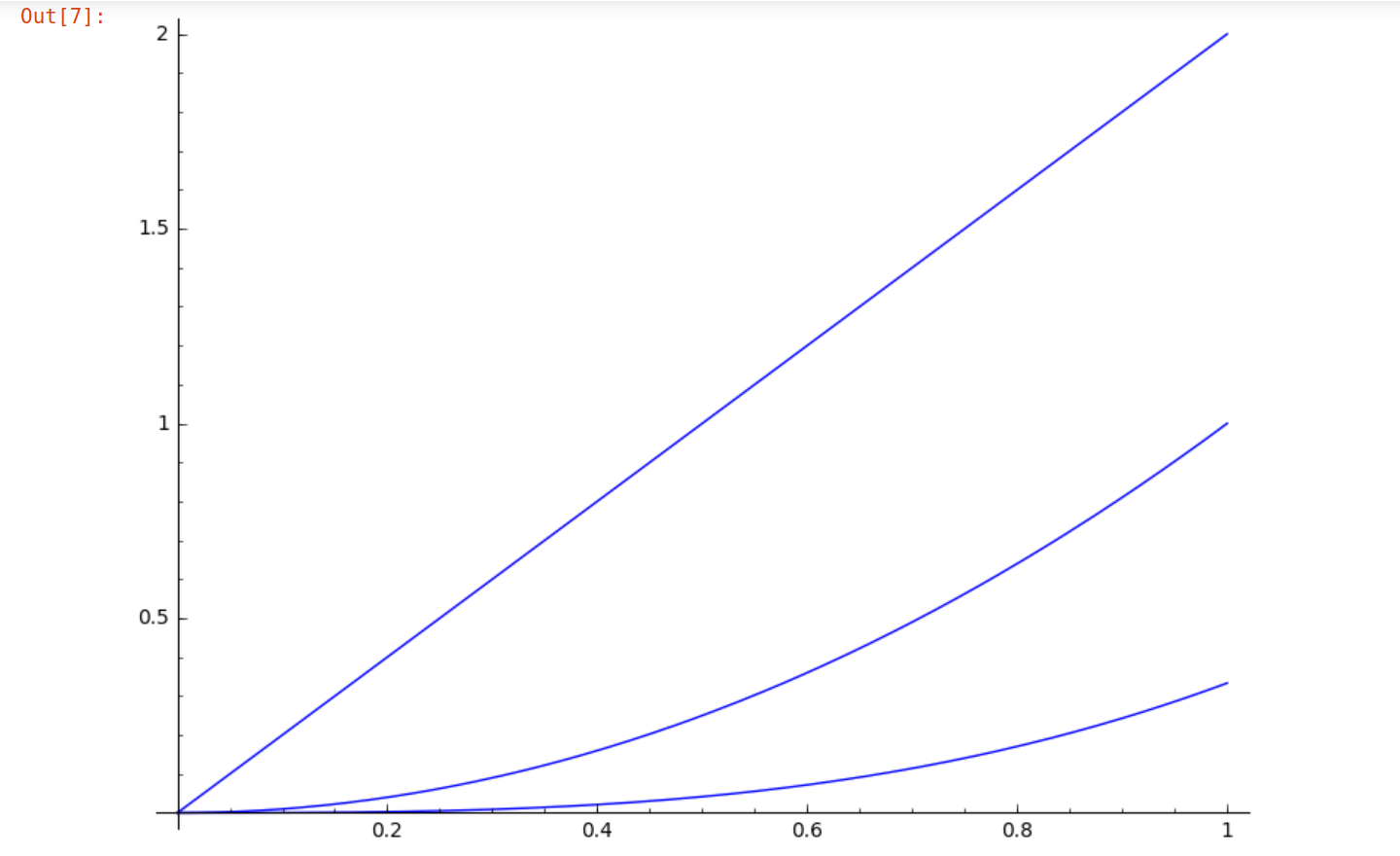
diff(x^3 + 3*x^2)3x^2 + 6x
integral(x*sin(2*x)*cos(x)^3, x)-1/40xcos(5x) - 1/8xcos(3x) - 1/4xcos(x) + 1/200sin(5x) + 1/24sin(3x) + 1/4*sin(x)
[∇] [Δ] Équations différentielles ordinaires
from sage.calculus.desolvers import desolve_odeint
t, x, y = var('t, x, y')
t   = srange(0, 10, 0.1)
f   = [x*(1-y), -y*(1-x)]
sol = desolve_odeint(f, [0.5,2], t, [x,y])
p   = line(zip(sol[:,0], sol[:,1]))
p.show() 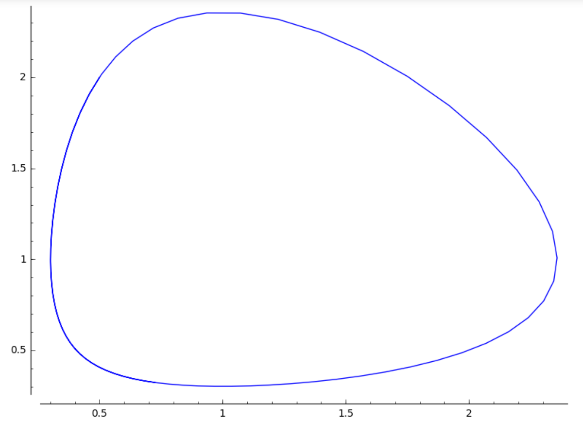
[∇] [Δ] Théorie des graphes
n = 6
G = graphs.CompleteGraph(n)
from sage.graphs.graph_coloring import edge_coloring
for jour, matches in enumerate(edge_coloring(G)) :
    print "Matches du jour " + str(jour) + " : " + str(matches)
Matches du jour 0 : [(0, 5), (1, 4), (2, 3)] Matches du jour 1 : [(0, 2), (1, 5), (3, 4)] Matches du jour 2 : [(0, 4), (1, 3), (2, 5)] Matches du jour 3 : [(0, 1), (2, 4), (3, 5)] Matches du jour 4 : [(0, 3), (1, 2), (4, 5)]
G = graphs.CompleteGraph(6)
G.show(edge_colors=edge_coloring(G, hex_colors=True)) 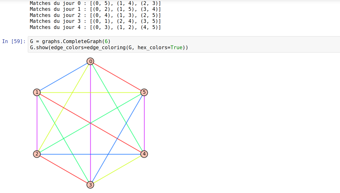
[∇] [Δ] Python : Fibonacci
#Copyright (C)   2007-2008   Creative Commons Attribution 2.5
#                            http://wiki.laptop.org/go/Pippy
#Version         2013-04-12  Jean.Thiery@ModLibre.info
#
#   Title:  Fibonacci Series
#   Author: Rafael Ortiz </go/User:RafaelOrtiz>
#   About:  The Fibonacci Number Series
#   en:     http://en.wikipedia.org/wiki/Fibonacci_number
#   fr:     http://fr.wikipedia.org/wiki/Suite_de_Fibonacci
#   Shows:  Using tuple assignments. While loop.

a, b = 0, 1
while b < 1001:
     print b,
     a, b = b, a+b

print
print
1 1 2 3 5 8 13 21 34 55 89 144 233 377 610 987
[∇] [Δ] Python : Fibonacci 2
#Copyright (C)   2007-2008   Creative Commons Attribution 2.5
#                            http://wiki.laptop.org/go/Pippy
#Version         2013-04-12  Jean.Thiery@ModLibre.info
#
#   Title:  Fibonacci Series (normal and alternate)
#   Author: Rafael Ortiz </go/User:RafaelOrtiz>
#   About:  The Fibonacci Number Series
#   en:     http://en.wikipedia.org/wiki/Fibonacci_number
#   fr:     http://fr.wikipedia.org/wiki/Suite_de_Fibonacci
#   Shows:  Using tuple assignments. While loop.

a, b = 0, 1
while b < 1001:
     print b,
     a, b = b, a+b

print

a, b = 0, 1
while b < 1001:
     print b,
     a, b = b, a-b

print
print
1 1 2 3 5 8 13 21 34 55 89 144 233 377 610 987 1 -1 2 -3 5 -8 13 -21 34 -55 89 -144 233 -377 610 -987
[∇] [Δ] Python : Triangle de Sierpinski
#Copyright (C)   2007-2008   Creative Commons Attribution 2.5
#                            http://wiki.laptop.org/go/Pippy
#Version         2013-04-12  Jean.Thiery@ModLibre.info
#
#   Title:  Sierpinski's triangle
#   Author: Madeleine Ball
#   About:  Character graphics of a Sierpinski triangle
#   en:     http://en.wikipedia.org/wiki/Sierpinski_triangle
#   fr:     http://fr.wikipedia.org/wiki/Triangle_de_Sierpi%C5%84ski
#   Shows:  Modifying Pascal's triangle program, loops, vectors

size = 4 # 5
modulus = 2

lines = modulus**size

vector = [1]
for i in range(1,lines+1):
  vector.insert(0,0)
  vector.append(0)

for i in range(0,lines):
  newvector = vector[:]
  for j in range(0,len(vector)-1):
    if (newvector[j] == 0):
      print " ",
    else:
      remainder = newvector[j] % modulus
      if (remainder == 0):
        print "O",  # "O" or "#"
      else:
        print "-",  # "." or "="
    newvector[j] = vector[j-1] + vector[j+1]
  print
  vector = newvector[:]

print
-
- -
- O -
- - - -
- O O O -
- - O O - -
- O - O - O -
- - - - - - - -
- O O O O O O O -
- - O O O O O O - -
- O - O O O O O - O -
- - - - O O O O - - - -
- O O O - O O O - O O O -
- - O O - - O O - - O O - -
- O - O - O - O - O - O - O - 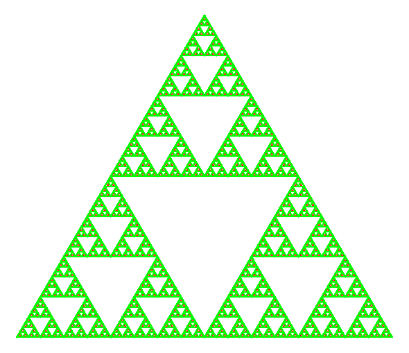
[∇] [Δ] Python : Tortue
from turtle import *
from math import *

AB = 50 * sqrt(13)
alpha = degrees(atan(2/3))
forward(200)
left(90)
forward(100)
left(90)
forward(50)
left(alpha)
forward(AB)

mainloop()
[∇] [Δ] Python : Lotka-Volterra
import scipy; from scipy import integrate
a, b, c, d = 1.0, 0.1, 1.5, 0.75
def dX_dt(X, t=0):                            # renvoie l'augmentation des populations
    return [ a * X[0] -     b * X[0] * X[1] ,
            -c * X[1] + d * b * X[0] * X[1] ]
t = srange(0, 15, 0.01)                       # échelle de temps
X0 = [10, 5]           # Conditions initiales : 10 lievres et 5 lynx
X  = integrate.odeint(dX_dt, X0, t)           # résolution numérique
lievres, lynx = X.T                           # raccourcis de X.transpose()
p  = line(zip(t, lievres),  color = 'green')  # tracé du nombre de lievres
p += line(zip(t, lynx), color='red')          # tracé du nombre de lynx
p.show() # tracé 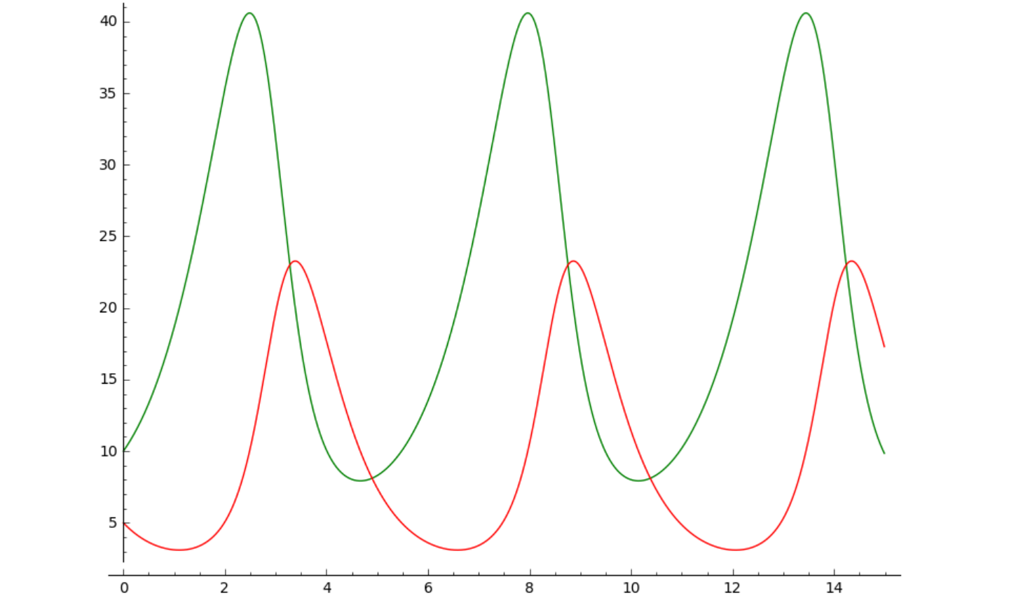
[∇] [Δ] Python : Lotka-Volterra + Libellés
import scipy; from scipy import integrate
a, b, c, d = 1.0, 0.1, 1.5, 0.75
def dX_dt(X, t=0):                            # renvoie l'augmentation des populations
    return [ a * X[0] -     b * X[0] * X[1] ,
            -c * X[1] + d * b * X[0] * X[1] ]
t = srange(0, 15, 0.01)                       # échelle de temps
X0 = [10, 5]           # Conditions initiales : 10 lievres et 5 lynx
X  = integrate.odeint(dX_dt, X0, t)           # résolution numérique
lievres, lynx = X.T                           # raccourcis de X.transpose()
p  = line(zip(t, lievres),  color = 'green')  # tracé du nombre de lievres
p += line(zip(t, lynx), color='red')          # tracé du nombre de lynx

p += text("Lievres",  (10.6, 37), fontsize = 20, color = 'green')
p += text("Lynx", (12,  8), fontsize = 20, color = 'red')
p.axes_labels(["temps", "population"]);
p.show(gridlines=True) # tracé 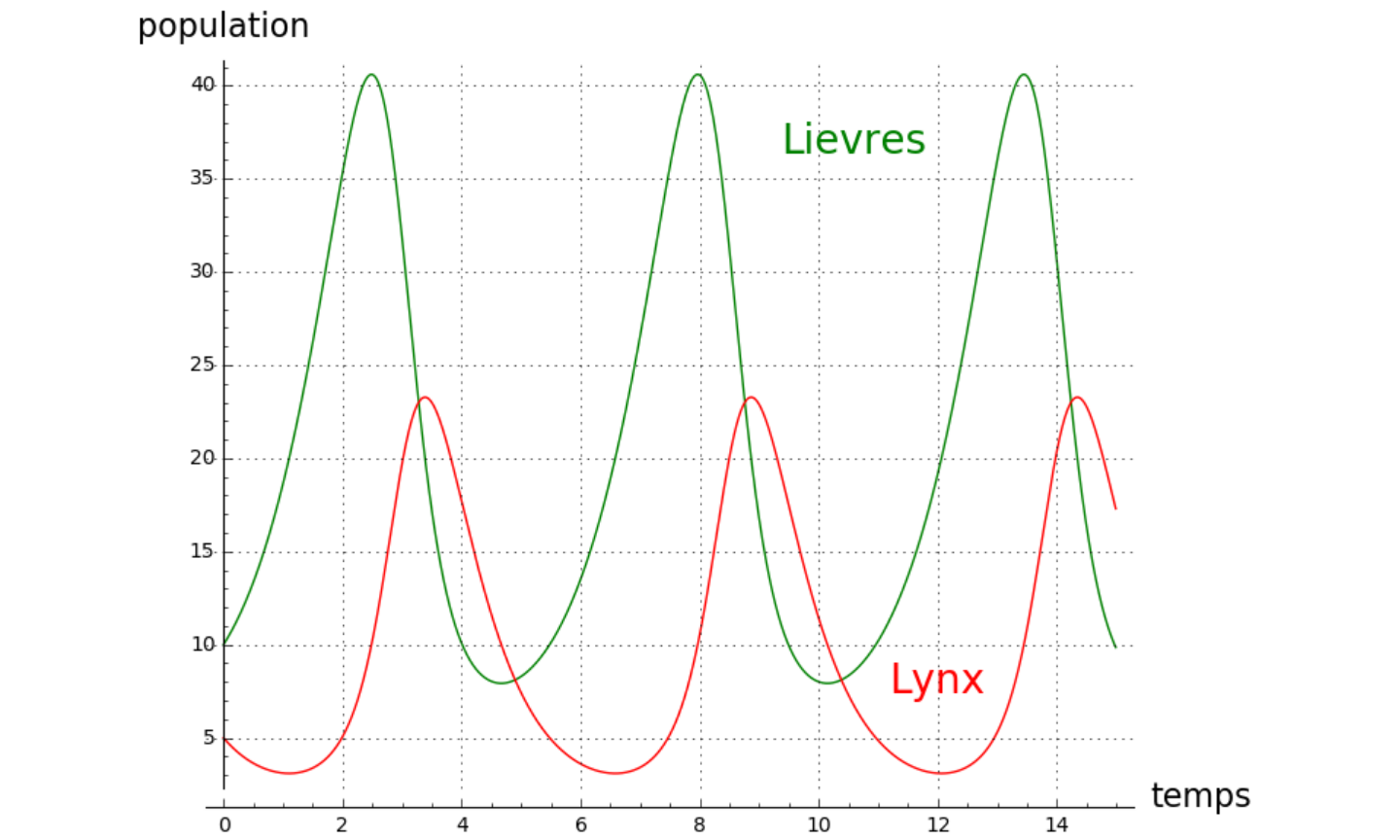
[∇] [Δ] Calculs divers : Langage R…
r.summary(r.c(1, 1, 2, 3, 5, 8, 13, 21, 34, 55, 89, 144, 233, 377, 610, 987))Min. 1st Qu. Median Mean 3rd Qu. Max. 1.0 4.5 27.5 161.4 166.2 987.0
Addition
1*200 + 2*50 + 8*20 + 3*10 + 7*5 + 1*2 + 3*1530
[∇] [Δ] Calculs interactifs
Vector Fields and Euler’s Method
x,y = var('x,y')
from sage.ext.fast_eval import fast_float
@interact
def _(f = input_box(default=y), g=input_box(default=-x*y+x^3-x),
      xmin=input_box(default=-1), xmax=input_box(default=1),
      ymin=input_box(default=-1), ymax=input_box(default=1),
      start_x=input_box(default=0.5), start_y=input_box(default=0.5),
      step_size=(0.01,(0.001, 0.2)), steps=(600,(0, 1400)) ):
    ff = fast_float(f, 'x', 'y')
    gg = fast_float(g, 'x', 'y')
    steps = int(steps)

    points = [ (start_x, start_y) ]
    for i in range(steps):
        xx, yy = points[-1]
        try:
            points.append( (xx + step_size * ff(xx,yy), yy + step_size * gg(xx,yy)) )
        except (ValueError, ArithmeticError, TypeError):
            break

    starting_point = point(points[0], pointsize=50)
    solution = line(points)
    vector_field = plot_vector_field( (f,g), (x,xmin,xmax), (y,ymin,ymax) )

    result = vector_field + starting_point + solution

    pretty_print(html(r"$\displaystyle\frac{dx}{dt} = %s$  $ \displaystyle\frac{dy}{dt} = %s$" % (latex(f),latex(g))))
    result.show(xmin=xmin,xmax=xmax,ymin=ymin,ymax=ymax)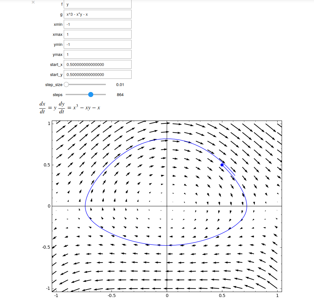

[∇] [Δ] Références
Calcul mathématique avec Sage A. Casamayou, N. Cohen, G. Connan, T. Dumont, L. Fousse, F. Maltey, M. Meulien, M. Mezzarobba, C. Pernet, N. M. Thiéry, P. Zimmermann : Licence libre CC-BY-SA 3.0; 468 pages, mai 2013, ISBN: 9781481191043
Computational Mathematics with SageMath Paul Zimmermann, Alexandre Casamayou, Nathann Cohen, Guillaume Connan, Thierry Dumont, Laurent Fousse, François Maltey, Matthias Meulien, Marc Mezzarobba, Clément Pernet, Nicolas M. Thiéry, Erik Bray, John Cremona, Marcelo Forets, Alexandru Ghitza, Hugh Thomas : Free license CC-BY-SA: xiv + 464 pages, December 2018